Hi everyone…
This post is continuation of my earlier post. In that post I have tried to cover basic concepts and terminologies used in estimation of population parameters. So if you are reading this first time I would recommend you to have a look at the earlier post.
So let us move ahead. Here we will discuss how to estimate population mean using sample mean (point estimate) w.r.t two situations
(a) when population standard deviation is known(using z-statistic).
(b) when population standard deviation is unknown(using t-statistic).
Case 1: When population standard deviation is known
Problem in hand : Suppose a large cellular phone company wants to meet the needs of cell phone users and for that they hire a research company to estimate the number of texts used per month by Americans in the 18-24 years of age category.
The research company studies the phone records of 85 randomly sampled Americans in the mentioned age category and computes a sample monthly mean of 1300 texts. Now we want to find the population mean.
Solution: If the cellular company uses the sample mean of 1300 texts as an estimate for the population mean, the sample mean is used as a point estimate. So let us look at the formula of computing z score to estimate the population mean. Here the level of confidence is 95% or alpha is 0.05
z = (x-μ)/σ
But since we are using point estimate we use standard error instead of using standard deviation directly. Standard error describes the typical error or uncertainty associated with the estimate.
Therefore the formula stands as:
z = (x-μ)/SE
z = (x-μ)/(σ/√n)
Rearranging this formula we get,
μ = x – (z *(σ/√n))
since we took our level of confidence as 95%, the level of error(α)permissible is 5%. Because a sample mean can be greater than or less than population mean, z can be negative or positive. So we would calculate the area on both sides of shaded areas from the center point 0. You can refer to the following diagram.
Therefore we can re-write the above expression as:
μ = x ± (Zα/2*(σ/√n)) equation(a)
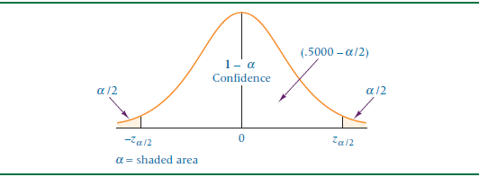
The value of Zα/2 or Z0.025 is found by looking in the standard normal table under 0.5000-0.0250 = 0.4750. This area in the table is associated with a z-value of 1.96
Also, suppose past history and similar studies indicate that population standard deviation is about 160.
Therefore,
x = 1300
Zα/2 = 1.96
σ = 160
n = 85
Putting all these values in the above equation we get,
μ = 1300 ± (1.96*(160/√85))
Solving it we will get,
1265.99 ≤ μ ≤ 1334.01 (This is our Confidence Interval)
So, the cellular telephone company researcher is 95% confident that the average number of texts per month by an American in the 18-24 year age category is between 1265.99 and 1334.01
To add one little thing which is very important is that, if your population is infinitely large and your sample size is less than 5% of your population you can use the equation(a) as it is, but if it is more than 5%, you should always one factor to the SE term called the “finite correction factor”. Equation(a) can be modified as :
μ = x ± (Zα/2*(σ/√n)*(√((N-1)/(N-n)))) equation(b)
where, N = size of the population.
In our above example, our population size was unknown and the sample size considered seems to be less than 5% of population size.
Finite Correction Factor reduces the width of the Confidence Interval. Less the width of Confidence Interval the more you tend towards accurate value of the population parameter.
Now, let us move on to the next case.
Case 2 : When population standard deviation is unknown
Suppose you are conducting your study for the first time and you do not have value for population standard deviation from studies conducted in the past. So how do you find the population parameter(here mean).
Yes, as we used sample mean as a point estimate, similarly we can use sample standard deviation as another point estimate. Everything else in equation(a) remains same. Instead of z-statistic we call it t-statistic. One assumption for using t-statistic is that the population should be normally distributed.
The formula for t-statistic is :
t = (x-μ)/(s/√n)
where,
x = sample mean
μ = population mean(to be estimated)
s = sample standard deviation
n = sample size
As we had z-table to calculate the values of z associated with some value of α, we also have a t-table here. To find a t-value associated with some area under t-curve, we need to understand one more term called “degrees of freedom”.
Degrees of freedom: It refers to the number of independent observations for a source of variation minus the number of independent parameters estimated in computing the variation.
Here, one independent parameter, population mean, μ, is being estimated by x (sample mean) in computing s. Thus, the degrees of freedom formula is n independent observations minus one independent parameter being estimated (n-1).
Therefore, the above equation can be re-written in terms of confidence interval as:
μ = x ± (tα/2,n-1*(s/√n)) equation(c)
Let us look at the following problem statement to understand how we can find population mean using t-statistic.
Problem: In aerospace industry some companies allow their employees to accumulate extra working hours beyond their 40 hour week. These extra hours are sometimes referred to as comp time. Suppose a researcher wants to estimate the average amount of comp time accumulated and per week for managers in the aerospace industry. The researcher randomly samples 18 managers and measures the amount of extra time they work during specific work. He constructs a 90% confidence interval to estimate the average amount of extra time per week worked by a manager in the aerospace industry.
Solution:
Sample size, n = 18
Degrees of freedom, n-1 = 17
α = 0.10, α/2 =0.05
x = 13.56 hours
s = 7.80 hours
From t-table in the above link we get
t0.05,17=1.740
Putting all the above values in equation(c) we get,
μ = 13.56 ± (1.740*(7.80/√18))
μ = 13.56 ± 3.20
10.36 ≤ μ ≤ 16.76
This means the researcher can be 90% confident that the average number of extra hours per week worked by a manager in the aerospace industry lies within 10.36 and 16.76 hours.
With this we come to an end of our post. I hope it was of some value to you. Please feel free to suggest or comment on this post. Give and take of knowledge always helps one to constantly improve.
Till we meet next time, Happy Learning!!!
References : Applied Business Statistics by Ken Black
Openintro.org
